5. Shape and symmetry
The last two sections showed how to model shape and symmetry individually, but we can be more creative and combine the two.
Download this page as a Jupyter notebook
5.1. Nanoribbons
To create a graphene nanoribbon, we’ll need a shape to give the finite width of the ribbon while the infinite length is achieved by imposing translational symmetry.
from pybinding.repository import graphene

model = pb.Model(
    graphene.monolayer(),
    pb.rectangle(1.2),  # nm
    pb.translational_symmetry(a1=True, a2=False)
)
model.plot()
model.lattice.plot_vectors(position=[-0.6, 0.3])  # nm
As before, the central darker circles represent the main cell of the nanoribbon, the lighter colored circles are the translations due to symmetry and the red lines are boundary hoppings. The two arrows in the upper left corner show the primitive lattice vectors of graphene.
The translational_symmetry() is applied only in the \(a_1\) lattice vector direction
which gives the ribbon its infinite length, but the symmetry is disabled in the \(a_2\)
direction so that the finite size of the shape is preserved. The builtin rectangle() shape
gives the nanoribbon its 1.2 nm width.
The band structure calculations work just as before.
from math import pi, sqrt

solver = pb.solver.lapack(model)
a = graphene.a_cc * sqrt(3)  # ribbon unit cell length
bands = solver.calc_bands(-pi/a, pi/a)
bands.plot()
This is the characteristic band structure for zigzag nanoribbons with zero-energy edge states. If we change the direction of the translational symmetry to \(a_2\), the orientation will change, but we will still have a zigzag nanoribbon.
model = pb.Model(
    graphene.monolayer(),
    pb.rectangle(1.2),  # nm
    pb.translational_symmetry(a1=False, a2=True)
)
model.plot()
model.lattice.plot_vectors(position=[0.6, -0.25])  # nm
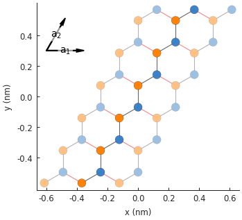
Because of the nature of graphene’s 2-atom unit cell and lattice vector, only zigzag edges can be created. In order to create armchair edges, we must introduce a different unit cell with 4 atoms.
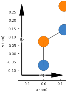
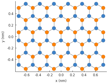
model = pb.Model(graphene.monolayer_4atom())
model.plot()
model.lattice.plot_vectors(position=[-0.13, -0.13])
Note
To learn how to create this 4-atom unit cell, see Constructing a supercell.
Notice that the lattice vectors \(a_1\) and \(a_2\) are at a right angle, unlike the sharp angle of the base 2-atom cell. The lattice properties are identical for the 2 and 4 atom cells, but the new geometry helps to create armchair edges.
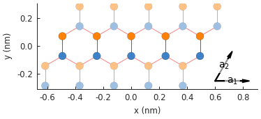
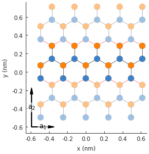
model = pb.Model(
    graphene.monolayer_4atom(),
    pb.primitive(a1=5),
    pb.translational_symmetry(a1=False, a2=True)
)
model.plot()
model.lattice.plot_vectors(position=[-0.59, -0.6])
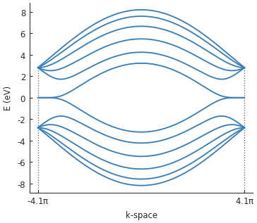
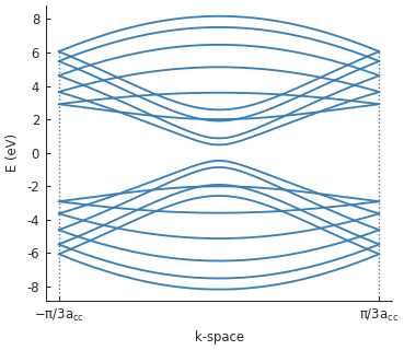
To calculate the band structure we must enter at least two points in k-space between which the
energy will be calculated. Note that because the periodicity is in the direction of the second
lattice vector \(a_2\), the points in k-space are given as [0, pi/d] instead of just
pi/d (which would be equivalent to [pi/d, 0]).
solver = pb.solver.lapack(model)
d = 3 * graphene.a_cc  # ribbon unit cell length
bands = solver.calc_bands([0, -pi/d], [0, pi/d])
bands.plot(point_labels=['$-\pi / 3 a_{cc}$', '$\pi / 3 a_{cc}$'])
5.2. 1D periodic supercell
Up to now, we used translational_symmetry() with True or False parameters to enable
or disable periodicity in certain directions. We can also pass a number to indicate the desired
period length.
model = pb.Model(
    graphene.monolayer_4atom(),
    pb.rectangle(x=2, y=2),
    pb.translational_symmetry(a1=1.2, a2=False)
)
model.plot()
The period length is given in nanometers. Note that our base shape is a square with 2 nm sides. The base shape forms the supercell of the periodic structure, but because the period length (1.2 nm) is smaller than the shape (2 nm), the extra length is cut off by the periodic boundary.
If you specify a periodic length which is larger than the base shape, the periodic conditions will not be applied because the periodic boundary will not have anything to bind to.
model = pb.Model(
    graphene.monolayer_4atom(),
    pb.rectangle(x=1.5, y=1.5),  # don't combine a small shape
    pb.translational_symmetry(a1=1.7, a2=False)  # with large period length
)
model.plot()
As you can see, making the period larger than the shape (1.7 nm vs. 1.5 nm), results in just the finite-sized part of the system. Don’t do this.
The combination of shape and symmetry can be more complex as shown here with a nanoribbon ring structure.
def ring(inner_radius, outer_radius):
    """Ring shape defined by an inner and outer radius"""
    def contains(x, y, z):
        r = np.sqrt(x**2 + y**2)
        return np.logical_and(inner_radius < r, r < outer_radius)
    return pb.FreeformShape(contains, width=[2*outer_radius, 2*outer_radius])

model = pb.Model(
    graphene.monolayer_4atom(),
    ring(inner_radius=1.4, outer_radius=2),
    pb.translational_symmetry(a1=3.8, a2=False)
)
plt.figure(figsize=[8, 3])
model.plot()
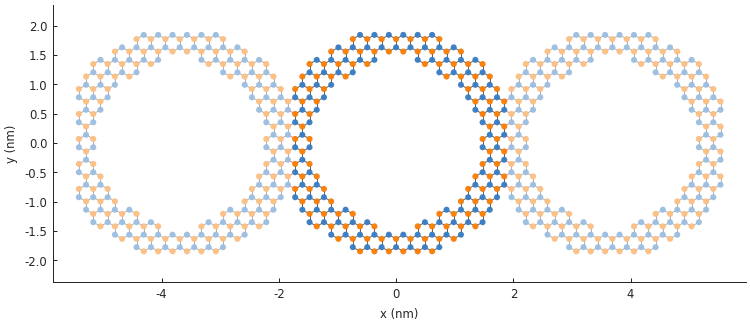
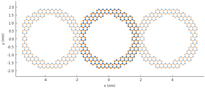
The period length of the translation in the \(a_1\) direction is set to 3.8 nm. This ensures that the inner ring shape is preserved and the periodic boundaries are placed on the outer edges.
solver = pb.solver.arpack(model, k=10) # only the 10 lowest states
a = 3.8  # [nm] unit cell length
bands = solver.calc_bands(-pi/a, pi/a)
bands.plot(point_labels=['$-\pi / a$', '$\pi / a$'])

5.3. 2D periodic supercell
A 2D periodic system made up of just a primitive cell was already covered in the Band structure
section. Here, we’ll create a system with a periodic unit cell which is larger than the primitive
cell. Similar to the 1D case, this is accomplished by giving translational_symmetry()
specific lengths for the translation directions. As an example, we’ll take a look at a graphene
antidot superlattice:
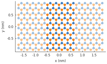
width = 2.5
rectangle = pb.rectangle(x=width * 1.2, y=width * 1.2)
dot = pb.circle(radius=0.4)

model = pb.Model(
    graphene.monolayer_4atom(),
    rectangle - dot,
    pb.translational_symmetry(a1=width, a2=width)
)
plt.figure(figsize=(5, 5))
model.plot()
model.lattice.plot_vectors(position=[2, -3.5], scale=3)
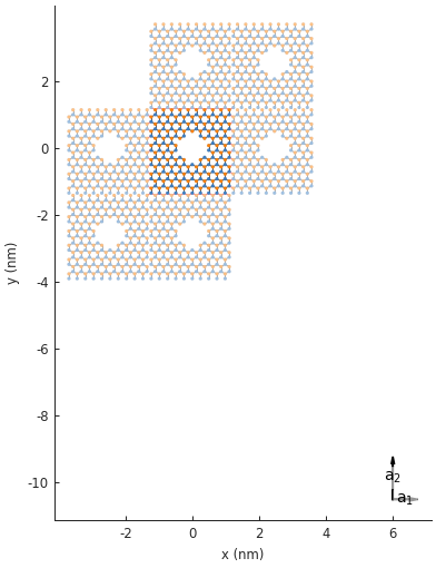
The antidot unit cell is created using a composite shape. Note that the
width of the rectangle is made to be slightly larger than the period length. Just like the 1D case,
this is necessary in order to give translational_symmetry() some room to cut off the edges
of the system and create periodic boundaries as needed. If the unit cell size is smaller then the
period length, translational symmetry cannot be applied.
In the figure above, notice that 6 translations of the unit cell are presented and it appears as
if 2 are missing. This is only in appearance. By default, Model.plot() shows just the
first-nearest translations of the unit cell. It just so happens that the 2 which appear missing
are second-nearest translations. To see this in the figure, we can set the num_periods argument
to a higher value:
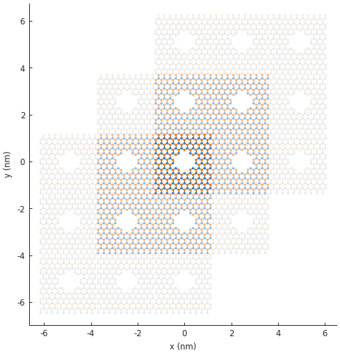
plt.figure(figsize=(5, 5))
model.plot(num_periods=2)
5.4. Example
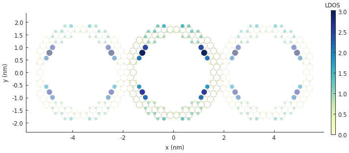
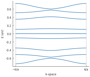
Note the zero-energy mode in the band structure. For wave vector \(k = 0\), states on the outer edge of the ring have the highest LDOS intensity, but for \(k = \pi / a\) the inner edge states dominate.
"""Model an infinite nanoribbon consisting of graphene rings"""
import pybinding as pb
import numpy as np
import matplotlib.pyplot as plt
from pybinding.repository import graphene
from math import pi

pb.pltutils.use_style()


def ring(inner_radius, outer_radius):
    """A simple ring shape"""
    def contains(x, y, z):
        r = np.sqrt(x**2 + y**2)
        return np.logical_and(inner_radius < r, r < outer_radius)

    return pb.FreeformShape(contains, width=[2 * outer_radius, 2 * outer_radius])


model = pb.Model(
    graphene.monolayer_4atom(),
    ring(inner_radius=1.4, outer_radius=2),  # length in nanometers
    pb.translational_symmetry(a1=3.8, a2=False)  # period in nanometers
)

plt.figure(figsize=pb.pltutils.cm2inch(20, 7))
model.plot()
plt.show()
# only solve for the 10 lowest energy eigenvalues
solver = pb.solver.arpack(model, k=10)
a = 3.8  # [nm] unit cell length
bands = solver.calc_bands(-pi/a, pi/a)
bands.plot(point_labels=[r'$-\pi / a$', r'$\pi / a$'])
plt.show()
solver.set_wave_vector(k=0)
ldos = solver.calc_spatial_ldos(energy=0, broadening=0.01)  # LDOS around 0 eV

plt.figure(figsize=pb.pltutils.cm2inch(20, 7))
ldos.plot(site_radius=(0.03, 0.12))
pb.pltutils.colorbar(label="LDOS")
plt.show()
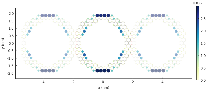
solver.set_wave_vector(k=pi/a)
ldos = solver.calc_spatial_ldos(energy=0, broadening=0.01)  # LDOS around 0 eV

plt.figure(figsize=pb.pltutils.cm2inch(20, 7))
ldos.plot(site_radius=(0.03, 0.12))
pb.pltutils.colorbar(label="LDOS")
plt.show()