7. Defects and strain
This section will introduce @site_state_modifier and
@site_position_modifier which can be used to add defects and
strain to the model. These modifiers are applied to the structure of the system before the
Hamiltonian matrix is created.
Download this page as a Jupyter notebook
7.1. Vacancies
A @site_state_modifier can be used to create vacancies in a crystal
lattice. The definition is very similar to the onsite and hopping modifiers explained in the
previous section.
def vacancy(position, radius):
    @pb.site_state_modifier
    def modifier(state, x, y):
        x0, y0 = position
        state[(x-x0)**2 + (y-y0)**2 < radius**2] = False
        return state
    return modifier
The state argument indicates the current boolean state of a lattice site. Only valid sites
(True state) will be included in the final Hamiltonian matrix. Therefore, setting the state of
sites within a small radius to False will exclude them from the final system. The x and y
arguments are lattice site positions. As with the other modifiers, the arguments are optional
(z is not needed for this example) but the full signature of the site state modifier can be
found on its API reference page.
This is actually very similar to the way a FreeformShape works. In fact, it is possible
to create defects by defining them directly in the shape. However, such an approach would not be
very flexible since we would need to create an entire new shape in order to change either the
vacancy type or the shape itself. By defining the vacancy as a modifier, we can simply compose
it with any existing shapes:
from pybinding.repository import graphene

model = pb.Model(
    graphene.monolayer(),
    pb.rectangle(2),
    vacancy(position=[0, 0], radius=0.1)
)
model.plot()
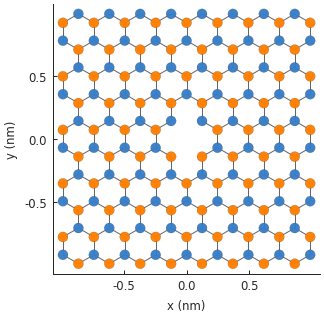
The resulting 2-atom vacancy is visible in the center of the system. The two vacant sites are
completely removed from the final Hamiltonian matrix. If we were to inspect the number of rows
and columns by looking up model.hamiltonian.shape, we would see that the size of the matrix is
reduced by 2.
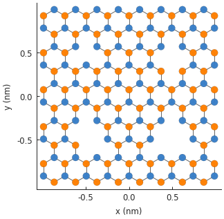
Any number of modifiers can be included in the model and they will compose as expected. We can take advantage of this and create four different vacancies, with 1 to 4 missing atoms:
model = pb.Model(
    graphene.monolayer(),
    pb.rectangle(2),
    vacancy(position=[-0.50,  0.50], radius=0.1),
    vacancy(position=[ 0.50,  0.45], radius=0.15),
    vacancy(position=[-0.45, -0.45], radius=0.15),
    vacancy(position=[ 0.50, -0.50], radius=0.2),
)
model.plot()
7.2. Layer defect
The site state modifier also has access to sublattice information. This can be used, for example,
with bilayer graphene to remove a single layer in a specific area. We’ll use the bilayer lattice
that’s included in the Material Repository. The graphene.bilayer()
lattice is laid out so that sublattices A1 and B1 belong to the top layer, while A2 and B2 are on
the bottom.
def scrape_top_layer(position, radius):
    """Remove the top layer of graphene in the area specified by position and radius"""
    @pb.site_state_modifier
    def modifier(state, x, y, sub_id):
        x0, y0 = position
        is_within_radius = (x-x0)**2 + (y-y0)**2 < radius**2
        is_top_layer = np.logical_or(sub_id == 'A1', sub_id == 'B1')
        final_condition = np.logical_and(is_within_radius, is_top_layer)
        state[final_condition] = False
        return state
    return modifier

model = pb.Model(
    graphene.bilayer(),
    pb.rectangle(2),
    scrape_top_layer(position=[0, 0], radius=0.5)
)
model.plot()
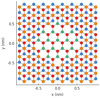
The central monolayer area is nicely visible in the figure. We can actually create the same
structure in a different way: by considering the z position of the lattice site to distinguish
the layers. An alternative modifier definition is given below. It would generate the same figure.
Which method is more convenient is up to the user.
def scrape_top_layer_alt(position, radius):
    """Alternative definition of `scrape_top_layer`"""
    @pb.site_state_modifier
    def modifier(state, x, y, z):
        x0, y0 = position
        is_within_radius = (x-x0)**2 + (y-y0)**2 < radius**2
        is_top_layer = (z == 0)
        final_condition = np.logical_and(is_within_radius, is_top_layer)
        state[final_condition] = False
        return state
    return modifier
Note
As with the onsite and hopping modifiers, all the arguments are given as numpy arrays.
Therefore, we must use the array-specific np.logical_or()/
np.logical_and() functions instead of the plain or/and
keywords.
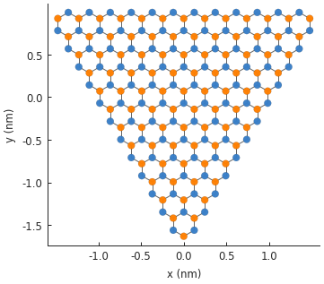
7.3. Strain
A @site_position_modifier can be used to model the lattice site
displacement caused by strain. Let’s start with a simple triangular system:
from math import pi

model = pb.Model(
    graphene.monolayer(),
    pb.regular_polygon(num_sides=3, radius=2, angle=pi),
)
model.plot()
We’re going to apply strain in three directions, as if we are pulling outward on the vertices of
the triangle. The displacement function for this kind of strain is given below. The c parameter
lets us control the intensity of the strain.
def triaxial_displacement(c):
    @pb.site_position_modifier
    def displacement(x, y, z):
        ux = 2*c * x*y
        uy = c * (x**2 - y**2)
        return x + ux, y + uy, z
    return displacement
The modifier function takes the x, y, z coordinates as arguments. The displacement ux, uy
is computed and the modified coordinates are returned. The z argument is returned unchanged but
we still need it here because the modifier is expected to always return all three.
model = pb.Model(
    graphene.monolayer(),
    pb.regular_polygon(num_sides=3, radius=2, angle=pi),
    triaxial_displacement(c=0.15)
)
model.plot()
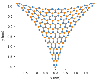
As seen in the figure, the displacement has been applied to the lattice sites and the new position data is saved in the system. However, the hopping energies have not been modified yet. Every hopping element of the Hamiltonian matrix is equal to the hopping energy of pristine graphene:
>>> np.all(model.hamiltonian.data == -2.8)
True
We now need to use the new position data to modify the hopping energy according to the relation
\(t = t_0 e^{-\beta (\frac{d}{a_{cc}} - 1)}\), where \(t_0\) is the original unstrained
hopping energy, \(\beta\) controls the strength of the strain-induced hopping modulation,
\(d\) is the strained distance between two atoms and \(a_{cc}\) is the unstrained
carbon-carbon distance. This can be implemented using a
@hopping_energy_modifier:
@pb.hopping_energy_modifier
def strained_hopping(energy, x1, y1, z1, x2, y2, z2):
    d = np.sqrt((x1-x2)**2 + (y1-y2)**2 + (z1-z2)**2)
    beta = 3.37
    w = d / graphene.a_cc - 1
    return energy * np.exp(-beta*w)
The structural modifiers (site state and position) are always automatically applied to the model
before energy modifiers (onsite and hopping). Thus, our strain_hopping modifier will get the new
displaced coordinates as its arguments, from which it will calculate the strained hopping energy.
model = pb.Model(
    graphene.monolayer(),
    pb.regular_polygon(num_sides=3, radius=2, angle=pi),
    triaxial_displacement(c=0.15),
    strained_hopping
)
Including the hopping modifier along with the displacement will yield position dependent hopping energy, thus the elements of the Hamiltonian will no longer be all equal:
>>> np.all(model.hamiltonian.data == -2.8)
False
However, it isn’t convenient to keep track of the displacement and strained hoppings separately. Instead, we can package them together in one function which is going to return both modifiers:
def triaxial_strain(c, beta=3.37):
    """Produce both the displacement and hopping energy modifier"""
    @pb.site_position_modifier
    def displacement(x, y, z):
        ux = 2*c * x*y
        uy = c * (x**2 - y**2)
        return x + ux, y + uy, z

    @pb.hopping_energy_modifier
    def strained_hopping(energy, x1, y1, z1, x2, y2, z2):
        l = np.sqrt((x1-x2)**2 + (y1-y2)**2 + (z1-z2)**2)
        w = l / graphene.a_cc - 1
        return energy * np.exp(-beta*w)

    return displacement, strained_hopping
The triaxial_strain function now has everything we need. We’ll apply it to a slightly larger
system so that we can clearly calculate the local density of states (LDOS). For more information
about this computation method see the Kernel polynomial method section. Right now, it’s enough to know that
we will calculate the LDOS at the center of the strained system, separately for sublattices
A and B.
model = pb.Model(
    graphene.monolayer(),
    pb.regular_polygon(num_sides=3, radius=40, angle=pi),
    triaxial_strain(c=0.0025)
)
kpm = pb.kpm(model)

for sub_name in ['A', 'B']:
    ldos = kpm.calc_ldos(energy=np.linspace(-1, 1, 500), broadening=0.03,
                         position=[0, 0], sublattice=sub_name)
    ldos.plot(label=sub_name, ls="--" if sub_name == "B" else "-")
pb.pltutils.legend()
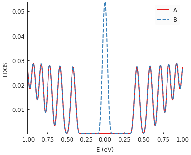
Strain in graphene has an effect similar to a magnetic field. That’s why we see Landau-level-like features in the LDOS. Note that the zero-energy peak has double intensity on one sublattice but zero on the other: this is a unique feature of the strain-induced pseudo-magnetic field.
7.4. Further reading
Take a look at the Modifiers API reference for more information.
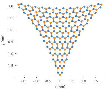
7.5. Example
"""Strain a triangular system by pulling on its vertices"""
import pybinding as pb
import numpy as np
import matplotlib.pyplot as plt
from pybinding.repository import graphene
from math import pi

pb.pltutils.use_style()


def triaxial_strain(c):
    """Strain-induced displacement and hopping energy modification"""
    @pb.site_position_modifier
    def displacement(x, y, z):
        ux = 2*c * x*y
        uy = c * (x**2 - y**2)
        return x + ux, y + uy, z

    @pb.hopping_energy_modifier
    def strained_hopping(energy, x1, y1, z1, x2, y2, z2):
        l = np.sqrt((x1-x2)**2 + (y1-y2)**2 + (z1-z2)**2)
        w = l / graphene.a_cc - 1
        return energy * np.exp(-3.37 * w)

    return displacement, strained_hopping


model = pb.Model(
    graphene.monolayer(),
    pb.regular_polygon(num_sides=3, radius=2, angle=pi),
    triaxial_strain(c=0.1)
)
model.plot()
plt.show()
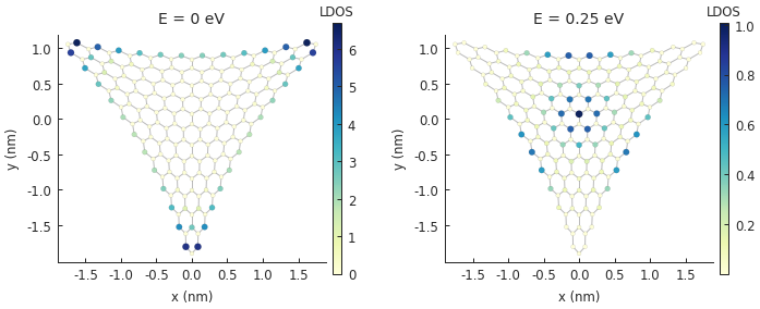
plt.figure(figsize=(7, 2.5))
grid = plt.GridSpec(nrows=1, ncols=2)
for block, energy in zip(grid, [0, 0.25]):
    plt.subplot(block)
    plt.title("E = {} eV".format(energy))

    solver = pb.solver.arpack(model, k=30, sigma=energy)
    ldos_map = solver.calc_spatial_ldos(energy=energy, broadening=0.03)
    ldos_map.plot()
    pb.pltutils.colorbar(label="LDOS")

plt.show()