10. Kernel polynomial method
The kernel polynomial method (KPM) can be used to quickly compute various physical properties
of very large tight-binding systems. It makes use of Chebyshev polynomial expansion together with
damping kernels. Pybinding includes a fast kpm() implementation with several easy-to-use
computation methods as well as a low-level interface for computing KPM expansion moments.
Download this page as a Jupyter notebook
10.1. About KPM
For a full review of the kernel polynomial method, see the reference paper Rev. Mod. Phys. 78, 275 (2006). Here, we shall only briefly describe the main characteristics of KPM and some specifics of its implementation in pybinding.
As we saw on the previous page, exactly solving a tight-binding problem implies the diagonalization of the Hamiltonian matrix. However, the computational resources required by eigenvalue solvers scale up rapidly with system size which makes it challenging to solve realistically large systems. A fundamentally different approach is to set aside the requirement for exact solutions (avoid diagonalization altogether) and instead use approximative methods to calculate the properties of interest. This is the main idea behind KPM which approximates functions as a series of Chebyshev polynomials.
The approximative nature of the method presents an opportunity for additional performance tuning. Results may be computed very quickly with low accuracy to get an initial estimate for the problem at hand. Once final results are required, the accuracy can be increased at the cost of longer computation time. Within pybinding, this KPM calculation quality is frequently expressed as an energy broadening parameter.
One of the great benefits of this method is that spatially dependent properties such as the local density of states (LDOS) or Green’s function are calculated separately for each spatial position. This means that localized properties can be computed extremely quickly. For this application, KPM can be seen as orthogonal to traditional eigenvalue solvers. Sparse diagonalization produces results for a very small energy range (eigenvalues) but does so for all positions simultaneously (eigenvectors). With KPM, it’s possible to separate and compute individual positions but for the entire energy spectrum at once. In this way, the two approaches complement each other nicely.
10.2. Builtin methods
Before using any of the computation methods, the main KPM object needs to be created
for a specific model:
model = pb.Model(...)
kpm = pb.kpm(model)
# ... use kpm
10.2.1. LDOS
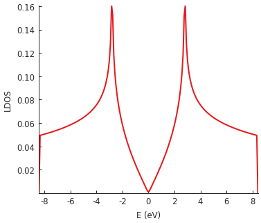
The KPM.calc_ldos() method makes it very easy to calculate the local density of states
(LDOS). In the next example we’ll use a large square sheet of pristine graphene:
from pybinding.repository import graphene

model = pb.Model(graphene.monolayer(), pb.rectangle(60, 60))
kpm = pb.kpm(model)

ldos = kpm.calc_ldos(energy=np.linspace(-9, 9, 200), broadening=0.05, position=[0, 0])
ldos.plot()
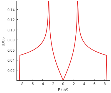
The LDOS is calculated for energies between -9 and 9 eV with a Gaussian broadening of 50 meV. Since this is the local density of states, position is also a required argument. We target the center of our square system where we expect to see the well-known LDOS shape of pristine graphene.
Thanks to KPM, the calculation of this local property is very fast: about 0.1 seconds for the example above with a 60 x 60 nm sheet of graphene. The broadening parameter offers the possibility for performance tuning – calculation time is inversely proportional to broadening width. KPM performs the computation for the entire spectrum simultaneously, so the selected energy range and the number of sample points have almost no effect on performance. The broadening width (i.e. the precision of the results) is the main factor which determines the duration of the calculation.
The result of the calculation is a Series object which contains the LDOS data, the energy
array for which it was calculated, and the associated data labels. This allows the
Series.plot() method to automatically plot a nicely labeled line plot, as seen above.
Accessing the raw data represented on the y-axis is possible via the Series.data
attribute, i.e. ldos.data in this specific case.
Tight-binding systems have lattice sites at discrete positions, which in principle means that we
cannot freely choose just any position for LDOS calculations. However, as a convenience the
KPM.calc_ldos() method will automatically find a valid site closest to the given target
position. We can optionally also choose a specific sublattice:
ldos = kpm.calc_ldos(energy=np.linspace(-9, 9, 200), broadening=0.05,
                     position=[0, 0], sublattice="B")
In this case we would calculate the LDOS at a site of sublattice B closest to the center of the system. We can try that on a graphene system with a mass term:
model = pb.Model(
    graphene.monolayer(),
    graphene.mass_term(1),
    pb.rectangle(60)
)
kpm = pb.kpm(model)

for sub_name in ["A", "B"]:
    ldos = kpm.calc_ldos(energy=np.linspace(-9, 9, 500), broadening=0.05,
                         position=[0, 0], sublattice=sub_name)
    ldos.plot(label=sub_name)
pb.pltutils.legend()
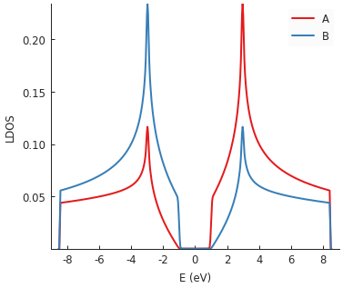
Multiple plots compose nicely here. A large band gap is visible at zero energy due to the inclusion
of graphene.mass_term(). It places an onsite potential with
the opposite sign in each sublattice. This is also why the LDOS lines for A and B sublattices are
antisymmetric around zero energy with respect to one another.
10.2.2. DOS
The following example demonstates the usage of the KPM.calc_dos() method which computes
the total density of states (DOS) in a system:
model = pb.Model(graphene.monolayer(), pb.rectangle(400, 2))
kpm = pb.kpm(model)

dos = kpm.calc_dos(energy=np.linspace(-2.7, 2.7, 500), broadening=0.06, num_random=16)
dos.plot()
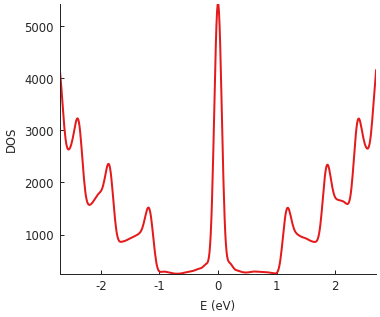
The example system here is a very long but narrow (400 x 2 nm) rectangle of graphene, i.e. a zigzag nanoribbon of finite length. The pronounced zero-energy peak is due to zigzag edge states and the additional higher-energy DOS peaks reflect the quantized band structure of the narrow nanoribbon.
A specific feature of the KPM-based DOS calculation is that it can be approximated very quickly
using stochastic methods. Instead of computing the density of states at each sites individually
and summing up the results, the DOS is calculated for all sites at the same time, but with a random
contribution of each site. By repeating this procedure multiple times with different random staring
states, the full DOS is recovered. This presents an additional knob for performance/quality tuning
via the num_random parameter.
For this example, we keep num_random low to keep the calculation time under 1 second. Increasing
this number would smooth out the DOS further. Luckily, the stochastic evaluation converges as a
function of both the system size and number of random samples. Thus, the larger the model system,
the smaller num_random needs to be for the same result quality.
10.2.3. Spatial LDOS
To see the spatial distribution of the density of states, we could call the KPM.calc_ldos()
method for several positions and populate a SpatialMap. However, this would be tedious and
slow, so instead we have KPM.calc_spatial_ldos() which makes this much simpler. Let’s use
a strained bit of graphene as an example:
def gaussian_bump_strain(height, sigma):
    """Out-of-plane deformation (bump)"""
    @pb.site_position_modifier
    def displacement(x, y, z):
        dz = height * np.exp(-(x**2 + y**2) / sigma**2)  # gaussian
        return x, y, z + dz  # only the height changes

    @pb.hopping_energy_modifier
    def strained_hoppings(energy, x1, y1, z1, x2, y2, z2):
        d = np.sqrt((x1-x2)**2 + (y1-y2)**2 + (z1-z2)**2)  # strained neighbor distance
        return energy * np.exp(-3.37 * (d / graphene.a_cc - 1))  # see strain section

    return displacement, strained_hoppings

model = pb.Model(graphene.monolayer().with_offset([-graphene.a / 2, 0]),
                 pb.regular_polygon(num_sides=6, radius=4.5),
                 gaussian_bump_strain(height=1.6, sigma=1.6))

plt.figure(figsize=(6.7, 2.2))
plt.subplot(121, title="xy-plane", ylim=[-5, 5])
model.plot()
plt.subplot(122, title="xz-plane")
model.plot(axes="xz")
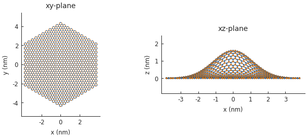
The bump produces purely out-of-plane strain so the xy-plane does not show any signs of the deformation. Switching to the xz-plane reveals the bump.
The KPM.calc_spatial_ldos() method takes the same energy and broadening arguments as
we’ve seen before. KPM computes the entire spectrum simultaneously, so it’s practically “free”
to compute the spatial LDOS at multiple energy values in one calculation (this is in contrast
to Solver.calc_spatial_ldos() which only targets a single energy).
The shape argument specifies the area where the LDOS is to be calculated, i.e. the sites which
are contained within the given shape. We could just specify the same shape as the model, thus
taking all sites into consideration, but the calculation is faster for smaller areas so we’ll
narrow our focus. Our model shape is hexagonal, but we’re only interested in the LDOS at the bump
so we can look at a smaller circular area:
kpm = pb.kpm(model)
spatial_ldos = kpm.calc_spatial_ldos(energy=np.linspace(-3, 3, 100), broadening=0.2,  # eV
                                     shape=pb.circle(radius=2.8))  # only within the shape
plt.figure(figsize=(6.7, 6))
gridspec = plt.GridSpec(2, 2, height_ratios=[1, 0.3], hspace=0)

energies = [0.0, 0.75, 0.0, 0.75]  # eV
planes = ["xy", "xy", "xz", "xz"]

for g, energy, axes in zip(gridspec, energies, planes):
    plt.subplot(g, title="E = {} eV, {}-plane".format(energy, axes))
    smap = spatial_ldos.structure_map(energy)
    smap.plot(site_radius=(0.02, 0.15), axes=axes)
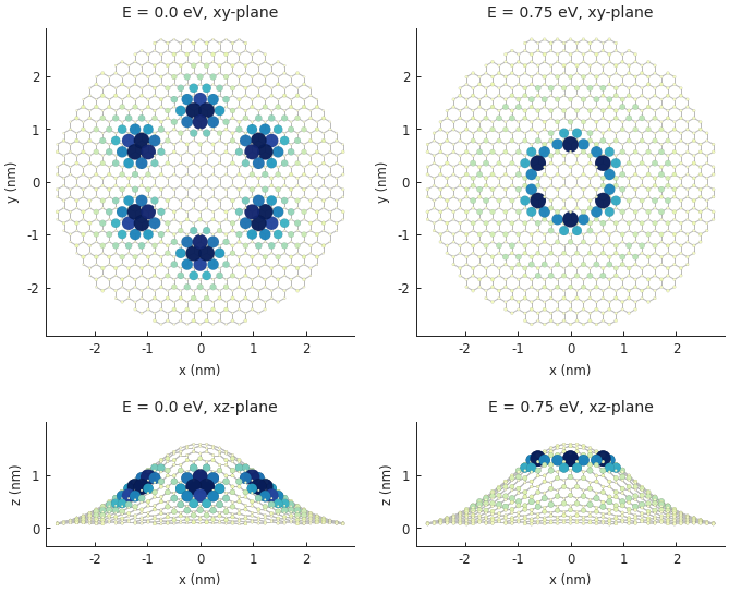
The result of the calculation is a SpatialLDOS object which stores the
spatial LDOS for several energy values. Calling SpatialLDOS.structure_map() selects
a specific energy.
10.2.4. Green’s function
The KPM.calc_greens() can then be used to calculate Green’s function corresponding to
Hamiltonian matrix element i,j for the desired energy range and broadening:
g_ij = kpm.calc_greens(i, j, energy=np.linspace(-9, 9, 100), broadening=0.1)
The result is raw Green’s function data for the given matrix element.
10.2.5. Conductivity
The KPM.calc_conductivity() method computes the conductivity as a function of chemical
potential. The implementation uses the Kubo-Bastin formula expanded in terms of Chebyshev
polynomials, as described in https://doi.org/10.1103/PhysRevLett.114.116602. The following
example calculates the conductivity tensor for the quantum Hall effect in graphene with
a magnetic field:
width = 40  # nanometers
model = pb.Model(
    graphene.monolayer(), pb.rectangle(width, width),
    graphene.constant_magnetic_field(magnitude=1500)  # exaggerated field strength
)

# The conductivity calculation is based on Green's function
# for which the Lorentz kernel produces better results.
kpm = pb.chebyshev.kpm(model, kernel=pb.lorentz_kernel())

directions = {
    r"$\sigma_{xx}$": "xx",  # longitudinal conductivity
    r"$\sigma_{xy}$": "xy",  # off-diagonal (Hall) conductivity
}
for name, direction in directions.items():
    sigma = kpm.calc_conductivity(chemical_potential=np.linspace(-1.5, 1.5, 300),
                                  broadening=0.1, direction=direction, temperature=0,
                                  volume=width**2, num_random=10)
    sigma.data *= 4  # to account for spin and valley degeneracy
    sigma.plot(label=name)
pb.pltutils.legend()
Note
The calculation above takes about a minute to complete. Please take note of that if you’ve downloaded this page as a Jupyter notebook and are executing the code on your own computer. If you’re viewing this online, you’ll notice that the result figure is not shown. This is because all of the figures in pybinding’s documentation are generated automatically by readthedocs.org (RTD) from the example code (not when you load the webpage, but when a new documentation revision is uploaded). RTD has a documentation build limit of 15 minutes so all of the example code presented on these pages is kept short and fast, preferably under 1 second for each snippet. The long runtime of this conductivity calculation forces us to skip it in order to conserve documentation build time.
You can execute this code on your own computer to see the results. The parameters here have been tuned in order to take the minimal amount of time while still showing the desired effect. However, that is not the most aesthetically pleasing result. To improve the quality of the resulting figure, you can increase the size of the system, reduce the magnetic field strength, reduce the broadening and increase the number of random vectors. That could extend the computation time from a few minutes to several hours.
10.3. Damping kernels
KPM approximates a function as a series of Chebyshev polynomials. This series is infinite, but numerical calculations must end at some point, thus taking into account only a finite number of terms. This truncation results in a loss of precision and high frequency oscillations in the computed function. In order to damp these fluctuations, the function can be convolved with various damping kernels (the K in KPM).
Pybinding offers three option: jackson_kernel(), lorentz_kernel() and
dirichlet_kernel(). The Jackson kernel is enabled by default and it is the best choice
for most applications. The following example compares the three kernels:
plt.figure(figsize=(6.7, 2.8))
model = pb.Model(graphene.monolayer(), pb.circle(30),
                 graphene.constant_magnetic_field(400))

plt.subplot(121, title="Damping kernels")
kernels = {"Jackson (default)": pb.jackson_kernel(),
           "Lorentz": pb.lorentz_kernel()}
for name, kernel in kernels.items():
    kpm = pb.kpm(model, kernel=kernel)
    ldos = kpm.calc_ldos(np.linspace(-1.5, 1.5, 500), broadening=0.05, position=[0, 0])
    ldos.plot(label=name, ls="--" if name == "Lorentz" else "-")
pb.pltutils.legend()

plt.subplot(122, title="Undamped")
kpm = pb.kpm(model, kernel=pb.dirichlet_kernel())
ldos = kpm.calc_ldos(np.linspace(-1.5, 1.5, 500), broadening=0.05, position=[0, 0])
ldos.plot(label="Dirichlet", color="C2")
pb.pltutils.legend()
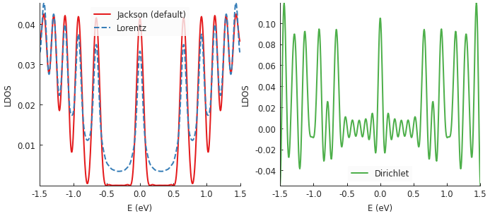
Computing the LDOS in graphene with a magnetic field reveals several peaks which correspond to
Landau levels. The Jackson kernel produces the best results. The broadening argument of the
calculation was set to 50 meV. With the Jackson kernel, the LDOS appears as if it was convolved
with a Gaussian of that width. On the other hand, the Lorentz kernel applies an effective
Lorentzian broadening of the same 50 meV but produces poorer results (not as sharp) simply due
to the difference in slopes of the Gaussian and Lorentzian curves.
Lastly, there is the Dirichlet kernel. It essentially doesn’t apply any damping and represent the raw result of the truncated Chebyshev series. Note that the Landau levels are still present, but there are also lots of extra oscillations (noise). The Dirichlet kernel is here mainly for demonstration purposes and is rarely useful.
Out of the two proper kernels, Jackson is the default and appropriate for most applications. The Lorentz kernels is mostly suited for Green’s function (and thus also conductivity) or in cases where the extra smoothing of the Lorentzian may be preferable (sometimes purely aesthetically).
10.4. Low-level interface
The KPM-based calculation methods presented so far have been user-friendly and aimed at computing
a single physical property of a model. Pybinding also offers a low-level KPM interface via the
KPM.moments() method. It can be used to generally compute KPM expansion moments of the
form \(\mu_n = <\beta|op \cdot T_n(H)|\alpha>\). For more information on how to use these
moments to reconstruct various functions, see Rev. Mod. Phys. 78, 275 (2006)
which explains everything in great detail.
We’ll just leave a quick example here. The following code calculates the LDOS in the center of a rectangular graphene flake. This is exactly like the first example in the LDOS section above, except that we are using the low-level interface. There is no special advantage to doing this calculation manually (in fact, the high-level method is faster). This is here simply for demonstration. The intended usage of the low-level interface is to create KPM-based computation methods which are not already covered by the builtins described above.
model = pb.Model(graphene.monolayer(), pb.rectangle(60, 60))
kpm = pb.kpm(model, kernel=pb.jackson_kernel())

# Construct a unit vector which is equal to 1 at the position
# where we want to calculate the local density of states
idx = model.system.find_nearest(position=[0, 0], sublattice="A")
alpha = np.zeros(model.hamiltonian.shape[0])
alpha[idx] = 1

# The broadening and the kernel determine the needed number of moments
a, b = kpm.scaling_factors
broadening = 0.05  # (eV)
num_moments = kpm.kernel.required_num_moments(broadening / a)

# Main calculation
moments = kpm.moments(num_moments, alpha)  # optionally also takes beta and an operator

# Reconstruct the LDOS function
energy = np.linspace(-8.42, 8.42, 200)
scaled_energy = (energy - b) / a
ns = np.arange(num_moments)
k = 2 / (a * np.pi * np.sqrt(1 - scaled_energy**2))
chebyshev = np.cos(ns * np.arccos(scaled_energy[:, np.newaxis]))
ldos = k * np.sum(moments.real * chebyshev, axis=1)

plt.plot(energy, ldos)
plt.xlabel("E (eV)")
plt.ylabel("LDOS")
pb.pltutils.despine()
10.5. Further reading
For an additional examples see the Magnetic field subsection of Fields and effects as
well as the Strain modifier subsection of Defects and strain.
The reference page for the chebyshev submodule contains more information.