9. Eigenvalue solvers
Solvers were first introduced in the Band structure section and then used throughout the tutorial to
present the results of the various models we constructed. This section will take a more detailed
look at the concrete lapack() and arpack() eigenvalue solvers and their common
Solver interface.
Download this page as a Jupyter notebook
9.1. LAPACK
The Solver class establishes the interface of a solver within pybinding, but it does not
contain a concrete diagonalization routine. For this reason we never instantiate the plain solver,
only its implementations such as solver.lapack().
The LAPACK implementation works on dense matrices which makes it well suited only for small systems. However, a great advantage of this solver is that it always solves for all eigenvalues and eigenvectors of a Hamiltonian matrix. This makes it perfect for calculating the entire band structure of the bulk or nanoribbons, as has been shown several times in this tutorial.
Internally, this solver uses the scipy.linalg.eigh() function for dense Hermitian matrices.
See the solver.lapack() API reference for more details.
9.2. ARPACK
The solver.arpack() implementation works on sparse matrices which makes it suitable for
large systems. However, only a small subset of the total eigenvalues and eigenvectors can be
calculated. This tutorial already contains a few examples where the ARPACK solver was used, and
one more is presented below.
Internally, the scipy.sparse.linalg.eigsh() function is used to solve large sparse Hermitian
matrices. The first argument to solver.arpack() must be the pybinding Model, but
the following arguments are the same as eigsh(), so the solver routine
can be tweaked as desired. Rather than reproduce the full list of options here, we refer you to
the scipy eigsh() reference documentation. Here, we will focus on the
specific features of solvers within pybinding.
9.3. Solver interface
No matter which concrete solver is used, they all share a common Solver interface.
The two primary properties are eigenvalues and eigenvectors.
These are the raw results of the exact diagonalization of the Hamiltonian matrix.
>>> from pybinding.repository import graphene
>>> model = pb.Model(graphene.monolayer())
>>> model.hamiltonian.todense()
[[ 0.0 -2.8]
 [-2.8  0.0]]
>>> solver = pb.solver.lapack(model)
>>> solver.eigenvalues
[-2.8 2.8]
>>> solver.eigenvectors
[[-0.707 -0.707]
 [-0.707  0.707]]
The properties contain just the raw data. However, Solver also offers a few convenient
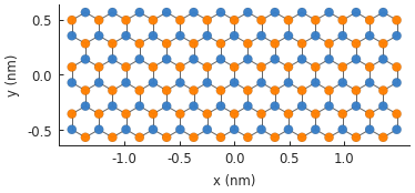
calculation methods. We’ll demonstrate these on a simple rectangular graphene system.
from pybinding.repository import graphene

model = pb.Model(
    graphene.monolayer(),
    pb.rectangle(x=3, y=1.2)
)
model.plot()
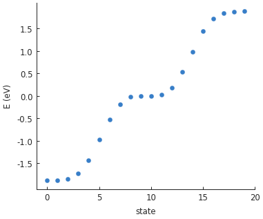
First, we’ll take a look at the calc_eigenvalues() method. While its job is
essentially the same as the eigenvalues property, there is one key difference:
the property returns a raw array, while the method returns an Eigenvalues result object.
These objects have convenient functions built in and they know how to plot their data:
solver = pb.solver.arpack(model, k=20)  # for the 20 lowest energy eigenvalues
eigenvalues = solver.calc_eigenvalues()
eigenvalues.plot()
The basic plot just shows the state number and energy of each eigenstate, but we can also do
something more interesting. If we pass a position argument to calc_eigenvalues()
it will calculate the probability density \(|\Psi(\vec{r})|^2\) at that position for each
eigenstate and we can view the result using Eigenvalues.plot_heatmap():
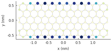
eigenvalues = solver.calc_eigenvalues(map_probability_at=[0.1, 0.6])  # position in [nm]
eigenvalues.plot_heatmap(show_indices=True)
pb.pltutils.colorbar()
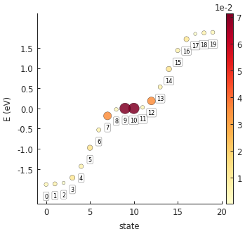
In this case we are interested in the probability density at [x, y] = [0.1, 0.6], i.e. a lattice
site at the top zigzag edge of our system. Note that the given position does not need to be
precise: the probability will be computed for the site closest to the given coordinates. From the
figure we can see that the probability at the edge is highest for the two zero-energy states:
numbers 9 and 10. We can take a look at the spatial map of state 9 using the
calc_probability() method:
probability_map = solver.calc_probability(9)
probability_map.plot()
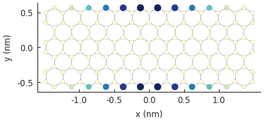
The result object in this case is a StructureMap with the probability density
\(|\Psi(\vec{r})|^2\) as its data attribute. As expected, the most prominent states are at
the zigzag edges of the system.
An alternative way to get a spatial map of the system is via the local density of states (LDOS).
The calc_spatial_ldos() method makes this easy. The LDOS map is requested for a
specific energy value instead of a state number and it considers multiple states within a Gaussian
function with the specified broadening:
ldos_map = solver.calc_spatial_ldos(energy=0, broadening=0.05)  # [eV]
ldos_map.plot()
The total density of states can be calculated with calc_dos():
dos = solver.calc_dos(energies=np.linspace(-1, 1, 200), broadening=0.05)  # [eV]
dos.plot()
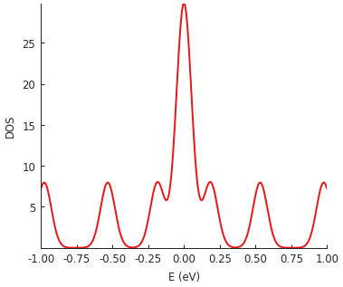
Our example system is quite small so the DOS does not resemble bulk graphene. The zero-energy peak stands out as the signature of the zigzag edge states.
For periodic systems, the wave vector can be controlled using Solver.set_wave_vector().
This allows us to compute the eigenvalues at various points in k-space. For example:
from math import pi

model = pb.Model(
    graphene.monolayer(),
    pb.translational_symmetry()
)
solver = pb.solver.lapack(model)

kx_lim = pi / graphene.a
kx_path = np.linspace(-kx_lim, kx_lim, 100)
ky_outer = 0
ky_inner = 2*pi / (3*graphene.a_cc)

outer_bands = []
for kx in kx_path:
    solver.set_wave_vector([kx, ky_outer])
    outer_bands.append(solver.eigenvalues)

inner_bands = []
for kx in kx_path:
    solver.set_wave_vector([kx, ky_inner])
    inner_bands.append(solver.eigenvalues)

for bands in [outer_bands, inner_bands]:
    result = pb.results.Bands(kx_path, bands)
    result.plot()
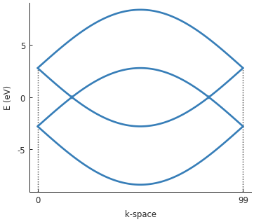
This example shows the basic principle of iterating over a path in k-space in order to calculate
the band structure. However, this is made much easier with the Solver.calc_bands() method.
This was already covered in the Band structure section and will not be repeated here. But keep in
mind that this calculation does not need to be done manually, Solver.calc_bands() is the
preferred way.
9.4. Further reading
Take a look at the solver and results reference pages for more detailed
information. More solver examples are available throughout this tutorial.