Lattice specification
This section covers a few extra features of the Lattice class. It is assumed that you
are already familiar with the Tutorial.
Download this page as a Jupyter notebook
First, we set a few constants which are going to be needed in the following examples:
from math import sqrt, pi

a = 0.24595   # [nm] unit cell length
a_cc = 0.142  # [nm] carbon-carbon distance
t = -2.8      # [eV] nearest neighbour hopping

Gamma = [0, 0]
K1 = [-4*pi / (3*sqrt(3)*a_cc), 0]
M = [0, 2*pi / (3*a_cc)]
K2 = [2*pi / (3*sqrt(3)*a_cc), 2*pi / (3*a_cc)]
Intrinsic onsite energy
During the construction of a Lattice object, the full signature of a sublattice is
(name, offset, onsite_energy=0.0), where the last argument is optional. The name and
offset arguments were already explained in the basic tutorial. The onsite_energy is applied
as an intrinsic part of the sublattice site. As an example, we’ll add this term to monolayer
graphene:
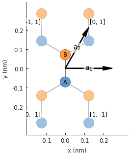
def monolayer_graphene(onsite_energy=[0, 0]):
    lat = pb.Lattice(a1=[a, 0], a2=[a/2, a/2 * sqrt(3)])
    lat.add_sublattices(('A', [0, -a_cc/2], onsite_energy[0]),
                        ('B', [0,  a_cc/2], onsite_energy[1]))
    lat.add_hoppings(([0,  0], 'A', 'B', t),
                     ([1, -1], 'A', 'B', t),
                     ([0, -1], 'A', 'B', t))
    return lat

lattice = monolayer_graphene()
lattice.plot()
Note
See Lattice.add_one_sublattice() and Lattice.add_sublattices().
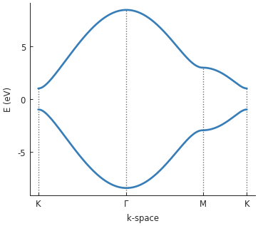
The effect of the onsite energy becomes apparent if we set opposite values for the A and B sublattices. This opens a band gap in graphene:
model = pb.Model(
    monolayer_graphene(onsite_energy=[-1, 1]),  # eV
    pb.translational_symmetry()
)
solver = pb.solver.lapack(model)
bands = solver.calc_bands(K1, Gamma, M, K2)
bands.plot(point_labels=['K', r'$\Gamma$', 'M', 'K'])
An alternative way of doing this was covered in the Opening a band gap section of the basic
tutorial. There, an @onsite_energy_modifier was used to produce
the same effect. The modifier is applied only after the system is constructed so it can depend on
the final (x, y, z) coordinates. Conversely, when the onsite energy is specified directly in a
Lattice object, it models an intrinsic part of the lattice and cannot depend on position.
If both the intrinsic energy and the modifier are specified, the values are added up.
Constructing a supercell
A primitive cell is the smallest unit cell of a crystal. For graphene, this is the usual 2-atom cell. It’s translated in space to construct a larger system. Sometimes it can be convenient to use a larger unit cell instead, i.e. a supercell consisting of multiple primitive cells. This allows us to slightly adjust the geometry of the lattice. For example, the 2-atom primitive cell of graphene has vectors at an acute angle with regard to each other. On the other hand, a 4-atom supercell is rectangular which makes certain model geometries easier to create. It also makes it possible to realize armchair edges, as shown in Nanoribbons section of the basic tutorial.
We can create a 4-atom cell by adding two more sublattice to the Lattice specification:
def monolayer_graphene_4atom():
    lat = pb.Lattice(a1=[a, 0], a2=[0, 3*a_cc])
    lat.add_sublattices(('A',  [  0, -a_cc/2]),
                        ('B',  [  0,  a_cc/2]),
                        ('A2', [a/2,    a_cc]),
                        ('B2', [a/2,  2*a_cc]))
    lat.add_hoppings(
        # inside the unit sell
        ([0, 0], 'A',  'B',  t),
        ([0, 0], 'B',  'A2', t),
        ([0, 0], 'A2', 'B2', t),
        # between neighbouring unit cells
        ([-1, -1], 'A', 'B2', t),
        ([ 0, -1], 'A', 'B2', t),
        ([-1,  0], 'B', 'A2', t),
    )
    return lat

lattice = monolayer_graphene_4atom()
plt.figure(figsize=(5, 5))
lattice.plot()
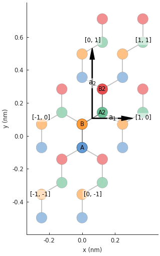
Note the additional sublattices A2 and B2, shown in green and red in the figure. As defined above,
these are interpreted as new and distinct lattice sites. However, we would like to have sublattices
A2 and B2 be equivalent to A and B. Lattice.add_aliases() does exactly that:
def monolayer_graphene_4atom():
    lat = pb.Lattice(a1=[a, 0], a2=[0, 3*a_cc])
    lat.add_sublattices(('A',  [  0, -a_cc/2]),
                        ('B',  [  0,  a_cc/2]))
    lat.add_aliases(('A2', 'A', [a/2, a_cc]),
                    ('B2', 'B', [a/2, 2*a_cc]))
    lat.add_hoppings(
        # inside the unit sell
        ([0, 0], 'A',  'B',  t),
        ([0, 0], 'B',  'A2', t),
        ([0, 0], 'A2', 'B2', t),
        # between neighbouring unit cells
        ([-1, -1], 'A', 'B2', t),
        ([ 0, -1], 'A', 'B2', t),
        ([-1,  0], 'B', 'A2', t),
    )
    return lat

lattice = monolayer_graphene_4atom()
plt.figure(figsize=(5, 5))
lattice.plot()
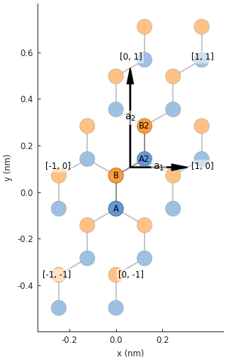
Now we have a supercell with only two unique sublattices: A and B. The 4-atom graphene unit cell is rectangular which makes it a more convenient building block than the oblique 2-atom cell.
Removing dangling bonds
When a finite-sized graphene system is constructed, it’s possible that it will contain a few
dangling bonds on the edge of the system. These are usually not desired and can be removed easily
by setting the Lattice.min_neighbors attribute:
plt.figure(figsize=(8, 3))
lattice = monolayer_graphene()
shape = pb.rectangle(x=1.4, y=1.1)

plt.subplot(121, title="min_neighbors == 1 -> dangling bonds")
model = pb.Model(lattice, shape)
model.plot()

plt.subplot(122, title="min_neighbors == 2", ylim=[-0.6, 0.6])
model = pb.Model(lattice.with_min_neighbors(2), shape)
model.plot()
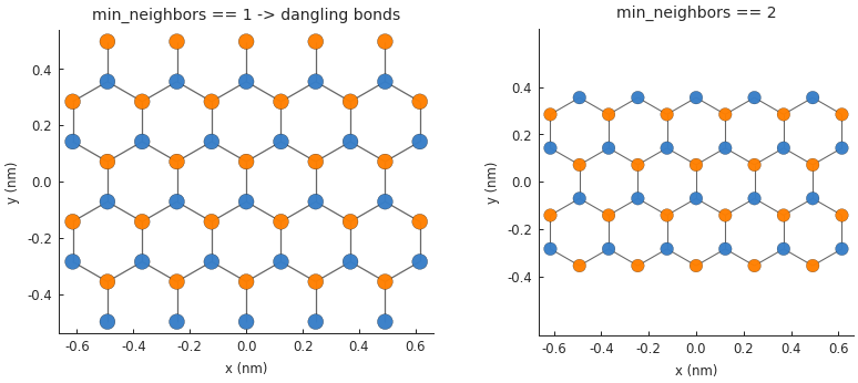
The dangling atoms on the edges have only one neighbor which makes them unique. When we use the
Lattice.with_min_neighbors() method, the model is required to remove any atoms which have
less than the specified minimum number of neighbors. Note that setting min_neighbors to 3
would produce an empty system since it is impossible for all atoms to have at least 3 neighbors.
Global lattice offset
When we defined monolayer_graphene() at the start of this section, we set the positions of the
sublattices as \([x, y] = [0, \pm a_{cc}]\), i.e. the coordinate system origin is at the
midpoint between A and B atoms. It can sometimes be convenient to choose a different origin
position such as the center of a hexagon formed by the carbon atoms. Rather than define an entirely
new lattice with different positions for A and B, we can simply offset the entire lattice by
setting the Lattice.offset attribute:
plt.figure(figsize=(8, 3))
shape = pb.regular_polygon(num_sides=6, radius=0.55)

plt.subplot(121, title="Origin between A and B atoms")
model = pb.Model(monolayer_graphene(), shape)
model.plot()
model.shape.plot()

plt.subplot(122, title="Origin in the center of a hexagon")
model = pb.Model(monolayer_graphene().with_offset([a/2, 0]), shape)
model.plot()
model.shape.plot()
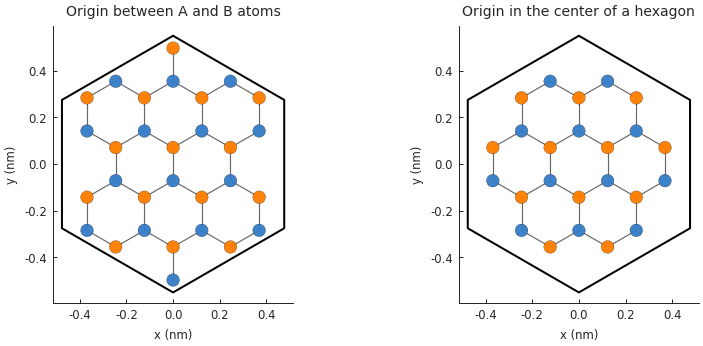
Note that the shape remains unchanged, only the lattice shifts position. We could have achieved the
same result by only moving the shape, but then the center of the shape would not match the origin
of the coordinate system. The Lattice.with_offset() makes it easy to position the lattice
as needed. Note that the given offset must be within half the length of a primitive lattice vector
(positive or negative). Beyond that length the lattice repeats periodically, so it doesn’t make
sense to shift it any father.
Position data types
By default, the data types for the positions are given in double. If you want to change this to float,
remove any existing pybinding installation by executing the following
command in terminal:
pip3 uninstall pybinding
Finally, reinstall it with float turned on:
PB_CARTESIAN_FLOAT=ON pip3 install pybinding --no-binary pybinding