4. Finite size

This section introduces the concept of shapes with classes Polygon and FreeformShape which are used to model systems of finite size. The sparse eigensolver arpack() is also introduced as a good tool for exactly solving larger Hamiltonian matrices.

Download this page as a Jupyter notebook

4.1. Primitive

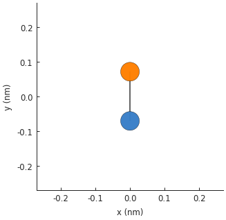
The simplest finite-sized system is just the unit cell of the crystal lattice.

from pybinding.repository import graphene

model = pb.Model(graphene.monolayer())
model.plot()

The unit cell can also be replicated a number of times to create a bigger system.

model = pb.Model(
    graphene.monolayer(),
    pb.primitive(a1=5, a2=3)
)
model.plot()
model.lattice.plot_vectors(position=[0.6, -0.25])

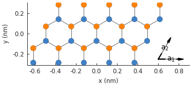
The primitive() parameter tells the model to replicate the unit cell 5 times in the \(a_1\) vector direction and 3 times in the \(a_2\) direction. However, to model realistic systems we need proper shapes.

4.2. Polygon

The easiest way to create a 2D shape is with the Polygon class. For example, a simple rectangle:

def rectangle(width, height):
    x0 = width / 2
    y0 = height / 2
    return pb.Polygon([[x0, y0], [x0, -y0], [-x0, -y0], [-x0, y0]])

shape = rectangle(1.6, 1.2)
shape.plot()

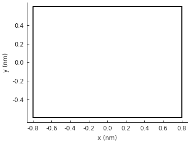
A Polygon is initialized with a list of vertices which should be given in clockwise or counterclockwise order. When added to a Model the lattice will expand to fill the shape.

model = pb.Model(
    graphene.monolayer(),
    rectangle(width=1.6, height=1.2)
)
model.plot()

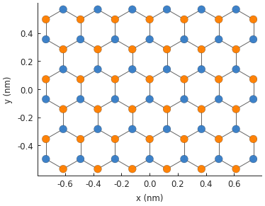
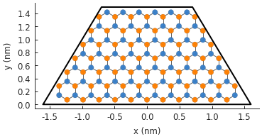
To help visualize the shape and the expanded lattice, the polygon outline can be plotted on top of the system by calling both plot methods one after another.

def trapezoid(a, b, h):
    return pb.Polygon([[-a/2, 0], [-b/2, h], [b/2, h], [a/2, 0]])

model = pb.Model(
    graphene.monolayer(),
    trapezoid(a=3.2, b=1.4, h=1.5)
)
model.plot()
model.shape.plot()

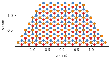
In general, a shape does not depend on a specific material, so it can be easily reused. Here, we shall switch to a graphene.bilayer() lattice, but we’ll keep the same trapezoid shape as defined earlier:

model = pb.Model(
    graphene.bilayer(),
    trapezoid(a=3.2, b=1.4, h=1.5)
)
model.plot()

4.3. Freeform shape

Unlike a Polygon which is defined by a list of vertices, a FreeformShape is defined by a contains function which determines if a lattice site is inside the desired shape.

def circle(radius):
    def contains(x, y, z):
        return np.sqrt(x**2 + y**2) < radius
    return pb.FreeformShape(contains, width=[2*radius, 2*radius])

model = pb.Model(
    graphene.monolayer(),
    circle(radius=2.5)
)
model.plot()

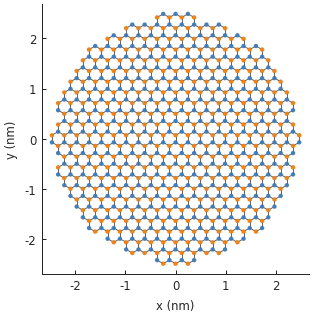
The width parameter of FreeformShape specifies the bounding box width. Only sites inside the bounding box will be considered for the shape. It’s like carving a sculpture from a block of stone. The bounding box can be thought of as the stone block, while the contains function is the carving tool that can give the fine detail of the shape.

As with Polygon, we can visualize the shape with the FreeformShape.plot() method.

def ring(inner_radius, outer_radius):
    def contains(x, y, z):
        r = np.sqrt(x**2 + y**2)
        return np.logical_and(inner_radius < r, r < outer_radius)
    return pb.FreeformShape(contains, width=[2*outer_radius, 2*outer_radius])

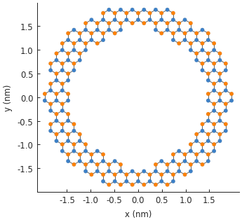
shape = ring(inner_radius=1.4, outer_radius=2)
shape.plot()

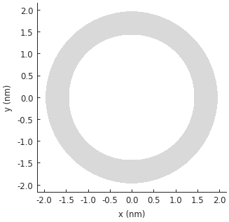
The shaded area indicates the shape as determined by the contains function. Creating a model will cause the lattice to fill in the shape.

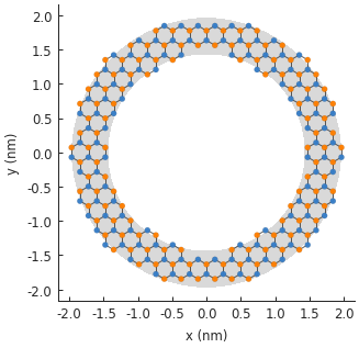
model = pb.Model(
    graphene.monolayer(),
    ring(inner_radius=1.4, outer_radius=2)
)
model.plot()
model.shape.plot()

Note that the ring example uses np.logical_and instead of the plain and keyword. This is because the x, y, z positions are not given as scalar numbers but as numpy arrays. Array comparisons return boolean arrays:

>>> x = np.array([7, 2, 3, 5, 1])
>>> x < 5
[False, True, True, False, True]
>>> 2 < x and x < 5
ValueError: ...
>>> np.logical_and(2 < x, x < 5)
[False, False, True, False, False]

The and keyword can only operate on scalar values, but np.logical_and can consider arrays. Likewise, math.sqrt does not work with arrays, but np.sqrt does.

4.4. Composite shape

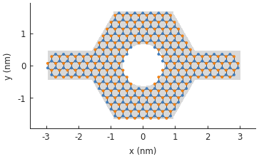
Complicated system geometry can also be produced by composing multiple simple shapes. The following example gives a quick taste of how it works. For a full overview of this functionality, see the Composite shapes section.

# Simple shapes
rectangle = pb.rectangle(x=6, y=1)
hexagon = pb.regular_polygon(num_sides=6, radius=1.92, angle=np.pi/6)
circle = pb.circle(radius=0.6)

# Compose them naturally
shape = rectangle + hexagon - circle

model = pb.Model(graphene.monolayer(), shape)
model.shape.plot()
model.plot()

4.5. Spatial LDOS

Now that we have a ring structure, we can exactly diagonalize its model.hamiltonian using a Solver. We previously used the lapack() solver to find all the eigenvalues and eigenvectors, but this is not efficient for larger systems. The sparse arpack() solver can calculate a targeted subset of the eigenvalues, which is usually desired and much faster. In this case, we are interested only in the 20 lowest energy states.

model = pb.Model(
    graphene.monolayer(),
    ring(inner_radius=1.4, outer_radius=2)
)
solver = pb.solver.arpack(model, k=20)  # only the 20 lowest eigenstates

ldos = solver.calc_spatial_ldos(energy=0, broadening=0.05)  # eV
ldos.plot(site_radius=(0.03, 0.12))
pb.pltutils.colorbar(label="LDOS")

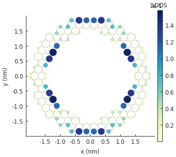
The convenient Solver.calc_spatial_ldos() method calculates the local density of states (LDOS) at every site for the given energy with a Gaussian broadening. The returned object is a StructureMap which holds the LDOS data. The StructureMap.plot() method will produce a figure similar to Model.plot(), but with a colormap indicating the LDOS value at each lattice site. In addition, the site_radius argument specifies a range of sizes which will cause the low intensity sites to appear as small circles while high intensity ones become large. The states with a high LDOS are clearly visible on the outer and inner edges of the graphene ring structure.

4.6. Further reading

For more finite-sized systems check out the examples section.

4.7. Example

Donwload source code

"""Model a graphene ring structure and calculate the local density of states"""
import pybinding as pb
import numpy as np
import matplotlib.pyplot as plt
from pybinding.repository import graphene

pb.pltutils.use_style()


def ring(inner_radius, outer_radius):
    """A simple ring shape"""
    def contains(x, y, z):
        r = np.sqrt(x**2 + y**2)
        return np.logical_and(inner_radius < r, r < outer_radius)

    return pb.FreeformShape(contains, width=[2 * outer_radius, 2 * outer_radius])


model = pb.Model(
    graphene.monolayer(),
    ring(inner_radius=1.4, outer_radius=2)  # length in nanometers
)

model.plot()
plt.show()

# only solve for the 20 lowest energy eigenvalues
solver = pb.solver.arpack(model, k=20)
ldos = solver.calc_spatial_ldos(energy=0, broadening=0.05)  # LDOS around 0 eV
ldos.plot(site_radius=(0.03, 0.12))
pb.pltutils.colorbar(label="LDOS")
plt.show()