6. Fields and effects
This section will introduce @onsite_energy_modifier and
@hopping_energy_modifier which can be used to add various
fields to the model. These functions can apply user-defined modifications to the Hamiltonian
matrix which is why we shall refer to them as modifier functions.
Download this page as a Jupyter notebook
6.1. Electric potential
We can define a simple potential function like the following:
@pb.onsite_energy_modifier
def potential(x, y):
    return np.sin(x)**2 + np.cos(y)**2
Here potential is just a regular Python function, but we attached a pretty @ decorator to it.
The @onsite_energy_modifier decorator gives an ordinary function
a few extra properties which we’ll talk about later. For now, just keep in mind that this is
required to mark a function as a modifier for use with pybinding models. The x and y
arguments are lattice site positions and the return value is the desired potential. Note the use
of np.sin instead of math.sin. The x and y coordinates are numpy arrays, not individual
numbers. This is true for all modifier arguments in pybinding. When you write modifier functions,
make sure to always use numpy operations which work with arrays, unlike regular math.
Note
Modifier arguments are passed as arrays for performance. Working with individual numbers would require calling the potential function individually for each lattice site which would be extremely slow. Arrays are much faster.
To use the potential function, just place it in a Model parameter list:
from pybinding.repository import graphene

model = pb.Model(
    graphene.monolayer(),
    pb.rectangle(12),
    potential
)
To visualize the potential, there’s the handy Model.onsite_map property which is a
StructureMap of the onsite energy of the Hamiltonian matrix.
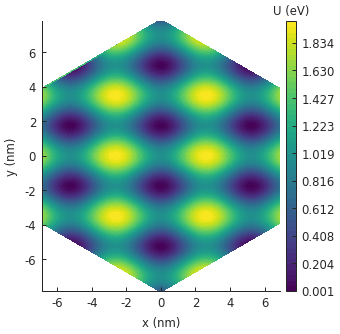
model.onsite_map.plot_contourf()
pb.pltutils.colorbar(label="U (eV)")
The figure shows a 2D colormap representation of our wavy potential in a square system. The
StructureMap.plot_contourf() method we just called is implemented in terms of matplotlib’s
contourf function with some slight adjustments for convenience.
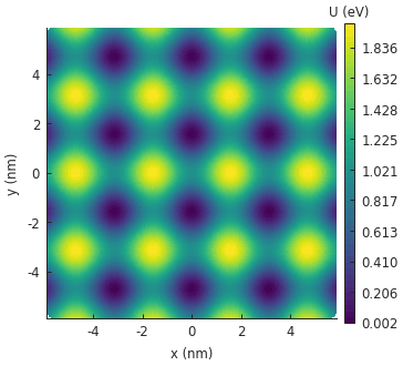
To make the potential more flexible, it’s a good idea to enclose it in an outer function, just like this:
def wavy(a, b):
    @pb.onsite_energy_modifier
    def potential(x, y):
        return np.sin(a * x)**2 + np.cos(b * y)**2
    return potential

model = pb.Model(
    graphene.monolayer(),
    pb.regular_polygon(num_sides=6, radius=8),
    wavy(a=0.6, b=0.9)
)
model.onsite_map.plot_contourf()
pb.pltutils.colorbar(label="U (eV)")
Note that we are using a system with hexagonal shape this time (via regular_polygon()).
The potential is only plotted inside the area of the actual system.
We can make one more improvement to our wavy function. We’ll add an energy argument:
def wavy2(a, b):
    @pb.onsite_energy_modifier
    def potential(energy, x, y):
        v = np.sin(a * x)**2 + np.cos(b * y)**2
        return energy + v
    return potential
The energy argument contains the existing onsite energy in the system before the new potential
function is applied. By adding to the existing energy, instead of just setting it, we can compose
multiple functions. For example, let’s combine the improved wavy2 with a linear potential.
def linear(k):
    @pb.onsite_energy_modifier
    def potential(energy, x):
        return energy + k*x
    return potential

model = pb.Model(
    graphene.monolayer(),
    pb.regular_polygon(num_sides=6, radius=8),
    wavy2(a=0.6, b=0.9),
    linear(k=0.2)
)
model.onsite_map.plot_contourf()
pb.pltutils.colorbar(label="U (eV)")
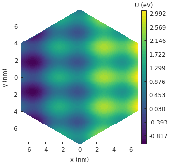
We see a similar wavy pattern as before, but the magnitude increases linearly along the x-axis
because of the contribution of the linear potential.
6.2. About the decorator
Now that you have a general idea of how to add and compose electric potentials in a model,
we should talk about the role of the @onsite_energy_modifier.
The full signature of a potential function looks like this:
@pb.onsite_energy_modifier
def potential(energy, x, y, z, sub_id):
    return ... # some function of the arguments
This function uses all of the possible arguments of an onsite energy modifier: energy, x,
y, z and sub_id. We have already explained the first three. The z argument is, obviously,
the z-axis coordinate of the lattice sites. The sub_id argument tells us which sublattice a site
belongs to. Its usage will be explained below.
As we have seen before, we don’t actually need to define a function to take all the arguments.
They are optional. The @ decorator will recognize a function which takes any of these arguments
and it will adapt it for use in a pybinding model. Previously, the linear function accepted only
the energy and x arguments, but wavy also included the y argument. The order of arguments
is not important, only their names are. Therefore, this is also a valid modifier:
@pb.onsite_energy_modifier
def potential(x, y, energy, sub_id):
    return ... # some function
But the argument names must be exact: a typo or an extra unknown argument will result in an error. The decorator checks this at definition time and decides if the given function is a valid modifier or not, so any errors will be caught early.
6.3. Opening a band gap
The last thing to explain about @onsite_energy_modifier is the
use of the sub_id argument. It tells us which sublattice a site belongs to. If you remember
from early on in the tutorial, in the process of specifying a lattice, we gave
each sublattice a unique name. This name can be used to filter out sites of a specific sublattice.
For example, let’s add mass to electrons in graphene:
def mass_term(delta):
    """Break sublattice symmetry with opposite A and B onsite energy"""
    @pb.onsite_energy_modifier
    def potential(energy, sub_id):
        energy[sub_id == 'A'] += delta
        energy[sub_id == 'B'] -= delta
        return energy
    return potential
Note that we don’t need x, y or z arguments because this will be applied everywhere evenly.
The mass_term function will add an energy delta to all sites on sublattice A and subtract
delta from all B sites. Note that we are indexing the energy array with a condition on the
sub_id array of the same length. This is a standard numpy indexing technique which you should
be familiar with.
The simplest way to demonstrate our new mass_term is with a graphene nanoribbon. First, let’s
just remind ourselves what a pristine zigzag nanoribbon looks like:
model = pb.Model(
    graphene.monolayer(),
    pb.rectangle(1.2),
    pb.translational_symmetry(a1=True, a2=False)
)
model.plot()
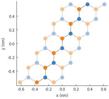
And let’s see its band structure:
from math import pi, sqrt

solver = pb.solver.lapack(model)
a = graphene.a_cc * sqrt(3)
bands = solver.calc_bands(-pi/a, pi/a)
bands.plot()
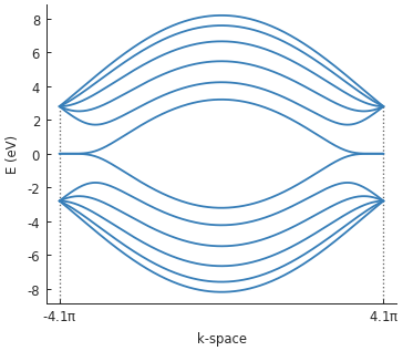
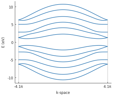
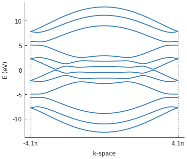
Note that the bands touch at zero energy: there is not band gap. Now, let’s include the mass term and compute the band structure again.
model = pb.Model(
    graphene.monolayer(),
    pb.rectangle(1.2),
    pb.translational_symmetry(a1=True, a2=False),
    mass_term(delta=2.5)  # eV
)
solver = pb.solver.lapack(model)
bands = solver.calc_bands(-pi/a, pi/a)
bands.plot()
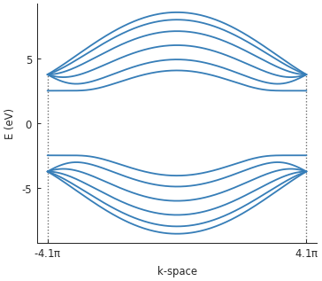
We set a very high delta value of 2.5 eV for illustration purposes. Indeed, a band gap of 5 eV
(delta * 2) is quite clearly visible in the band structure.
6.4. PN junction
While we’re working with a nanoribbon, let’s add a PN junction along its main axis.
def pn_junction(y0, v1, v2):
    @pb.onsite_energy_modifier
    def potential(energy, y):
        energy[y < y0] += v1
        energy[y >= y0] += v2
        return energy
    return potential
The y0 argument is the position of the junction, while v1 and v2 are the values of the
potential (in eV) before and after the junction. Let’s add it to the nanoribbon:
model = pb.Model(
graphene.monolayer(),
pb.rectangle(1.2),
pb.translational_symmetry(a1=True, a2=False),
pn_junction(y0=0, v1=-5, v2=5)
)
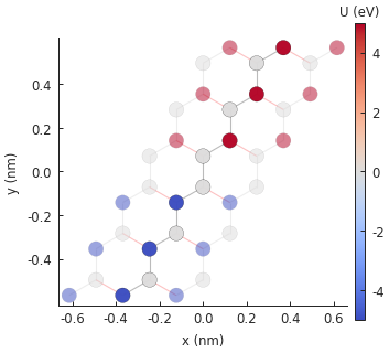
model.onsite_map.plot(cmap="coolwarm", site_radius=0.04)
pb.pltutils.colorbar(label="U (eV)")
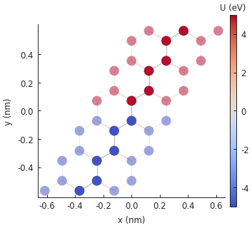
Remember that the Model.onsite_map property is a StructureMap, which has
several plotting methods. A contour plot would not look at all good for such a small nanoribbon,
but the method StructureMap.plot() is perfect. As before, the ribbon has infinite length
along the x-axis and the transparent sites represent the periodic boundaries. The PN junction
splits the ribbon in half along its main axis.
We can compute and plot the band structure:
solver = pb.solver.lapack(model)
bands = solver.calc_bands(-pi/a, pi/a)
bands.plot()
Next, let’s create a square potential well. We could define a new modifier function, as before. But lets take a different approach and create the well by composing two PN junctions.
model = pb.Model(
    graphene.monolayer(),
    pb.rectangle(1.2),
    pb.translational_symmetry(a1=True, a2=False),
    pn_junction(y0=-0.2, v1=5, v2=0),
    pn_junction(y0=0.2, v1=0, v2=5)
)
model.onsite_map.plot(cmap="coolwarm", site_radius=0.04)
pb.pltutils.colorbar(label="U (eV)")
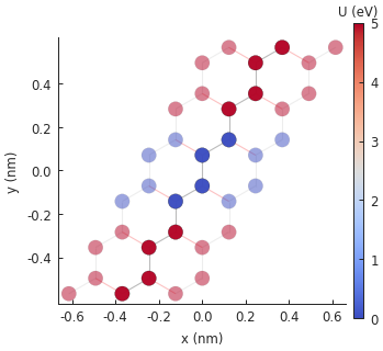
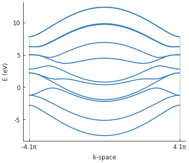
It works as expected. This can sometimes be a nice and quick way to extend a model. The square well affects the band structure by breaking electron-hole symmetry:
solver = pb.solver.lapack(model)
bands = solver.calc_bands(-pi/a, pi/a)
bands.plot()
6.5. Magnetic field
To model a magnetic field, we need to apply the Peierls substitution:
Here \(t_{nm}\) is the hopping energy between two sites, \(\Phi_0 = h/e\) is the magnetic quantum, \(h\) is the Planck constant and \(\vec{A}_{nm}\) is the magnetic vector potential along the path between sites \(n\) and \(m\). We want the magnetic field to be perpendicular to the graphene plane, so we can take the gauge \(\vec{A}(x,y,z) = (By, 0, 0)\).
This can all be expressed with a @hopping_energy_modifier:
from pybinding.constants import phi0

def constant_magnetic_field(B):
    @pb.hopping_energy_modifier
    def function(energy, x1, y1, x2, y2):
        # the midpoint between two sites
        y = 0.5 * (y1 + y2)
        # scale from nanometers to meters
        y *= 1e-9

        # vector potential along the x-axis
        A_x = B * y

        # integral of (A * dl) from position 1 to position 2
        peierls = A_x * (x1 - x2)
        # scale from nanometers to meters (because of x1 and x2)
        peierls *= 1e-9

        # the Peierls substitution
        return energy * np.exp(1j * 2*pi/phi0 * peierls)
    return function
The energy argument is the existing hopping energy between two sites at coordinates (x1, y1)
and (x2, y2). The function computes and returns the Peierls substitution as given by the
equation above.
The full signature of a @hopping_energy_modifier is actually:
@pb.hopping_energy_modifier
def function(energy, x1, y1, z1, x2, y2, z2, hop_id):
    return ... # some function of the arguments
The hop_id argument tells us which type of hopping it is. Hopping types can be specifically
named during the creation of a lattice. This can be used to apply functions only to specific
hoppings. However, as with all the modifier arguments, it’s optional, so we only take what we
need.
To test out our constant_magnetic_field, we’ll calculate the local density of states (LDOS),
where we expect to see peaks corresponding to Landau levels. The computation method used here
is explained in detail in the Kernel polynomial method section of the tutorial.
model = pb.Model(
    graphene.monolayer(),
    pb.rectangle(30),
    constant_magnetic_field(B=200)  # Tesla
)
kpm = pb.kpm(model)

ldos = kpm.calc_ldos(energy=np.linspace(-1, 1, 500), broadening=0.015, position=[0, 0])
ldos.plot()
plt.show()
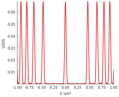
The values of the magnetic field is exaggerated here (200 Tesla), but that is done to keep the computation time low for the tutorial (less than 0.5 seconds for this LDOS calculation).
6.6. Further reading
Take a look at the Modifiers API reference for more information.
6.7. Example
"""PN junction and broken sublattice symmetry in a graphene nanoribbon"""
import pybinding as pb
import matplotlib.pyplot as plt
from pybinding.repository import graphene
from math import pi, sqrt

pb.pltutils.use_style()


def mass_term(delta):
    """Break sublattice symmetry with opposite A and B onsite energy"""
    @pb.onsite_energy_modifier
    def potential(energy, sub_id):
        energy[sub_id == 'A'] += delta
        energy[sub_id == 'B'] -= delta
        return energy

    return potential


def pn_juction(y0, v1, v2):
    """PN junction potential

    The `y0` argument is the position of the junction, while `v1` and `v2`
    are the values of the potential (in eV) before and after the junction.
    """
    @pb.onsite_energy_modifier
    def potential(energy, y):
        energy[y < y0] += v1
        energy[y >= y0] += v2
        return energy

    return potential


model = pb.Model(
    graphene.monolayer(),
    pb.rectangle(1.2),  # width in nanometers
    pb.translational_symmetry(a1=True, a2=False),
    mass_term(delta=2.5),  # eV
    pn_juction(y0=0, v1=-2.5, v2=2.5)  # y0 in [nm] and v1, v2 in [eV]
)
model.plot()
plt.show()

# plot the potential: note that pn_junction cancels out delta on some sites
model.onsite_map.plot(cmap="coolwarm", site_radius=0.04)
pb.pltutils.colorbar(label="U (eV)")
plt.show()
# compute the bands
solver = pb.solver.lapack(model)
a = graphene.a_cc * sqrt(3)  # nanoribbon unit cell length
bands = solver.calc_bands(-pi/a, pi/a)
bands.plot()
plt.show()