Kwant compatibility
Kwant is a Python package for numerical tight-binding similar to pybinding, but it’s specialized for transport calculations. Since the two packages work with the same kind of Hamiltonian matrices, it’s possible to build a model in pybinding and use Kwant to compute the transport properties. The advantage for pybinding users is access to Kwant’s transport solvers in addition to pybinding’s builtin computational routines. The advantage for Kwant users is the much faster system build times made possible by pybinding’s model builder – see the Benchmarks.
Download this page as a Jupyter notebook
Exporting a model
The procedure for constructing and solving transport problems in Kwant can be summarized with the following lines of pseudo-code:
# 1. BUILD model system
builder = kwant.Builder()
...  # specify model parameters
system = builder.finalized()

# 2. COMPUTE scattering matrix
smatrix = kwant.smatrix(system)
...  # call smatrix methods
If we want to use pybinding to build the model, we can just replace the first part:
# 1. BUILD model system
model = pb.Model(...)  # specify model parameters
kwant_system = model.tokwant()  # export to kwant format

# 2. COMPUTE scattering matrix
smatrix = kwant.smatrix(kwant_system)
...  # call smatrix methods
A pybinding Model is defined as usual and then converted to the Kwant-compatible format
by calling the Model.tokwant() method. The resulting kwant_system can be used as expected.
Complete example
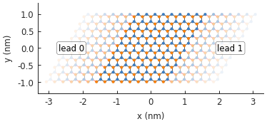
A detailed overview of scattering model construction in pybinding is available in the tutorial. Here, we present a simple example of a graphene wire with a potential barrier:
from pybinding.repository import graphene

def potential_barrier(v0, x0):
    """Barrier height `v0` in eV with spatial position `-x0 <= x <= x0`"""
    @pb.onsite_energy_modifier(is_double=True)  # enable double-precision floating-point
    def function(energy, x):
        energy[np.logical_and(-x0 <= x, x <= x0)] = v0
        return energy
    return function

def make_model(length, width, v0=0):
    model = pb.Model(
        graphene.monolayer(),
        pb.rectangle(length, width),
        potential_barrier(v0, length / 4)
    )
    model.attach_lead(-1, pb.line([-length/2, -width/2], [-length/2, width/2]))
    model.attach_lead(+1, pb.line([ length/2, -width/2], [ length/2, width/2]))
    return model

model = make_model(length=1, width=2)  # nm
model.plot()
We can then vary the height of the potential barrier and calculate the transmission using Kwant:
import kwant

length, width = 15, 15  # nm
electron_energy = 0.25  # eV
barrier_heights = np.linspace(0, 0.5, 100)  # eV

transmission = []
for v in barrier_heights:
    model = make_model(length, width, v)  # pybinding model
    kwant_system = model.tokwant()  # export to kwant
    smatrix = kwant.smatrix(kwant_system, energy=electron_energy)
    transmission.append(smatrix.transmission(1, 0))
For more information about kwant.smatrix and other transport calculations, please refer to the
Kwant website. That is outside the scope of this guide. The purpose
of this section is to present the Model.tokwant() compatibility method. The exported system
is then in the domain of Kwant.
From there, it’s trivial to plot the results:
plt.plot(barrier_heights, transmission)
plt.ylabel("transmission")
plt.xlabel("barrier height (eV)")
plt.axvline(electron_energy, 0, 0.5, color="gray", linestyle=":")
plt.annotate("electron energy\n{} eV".format(electron_energy), (electron_energy, 0.54),
             xycoords=("data", "axes fraction"), horizontalalignment="center")
pb.pltutils.despine()  # remove top and right axis lines
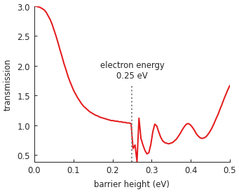
Note that the transmission was calculated for an energy value of 0.25 eV. As the height of the barrier is increased, two regimes are clearly distinguishable: transmission over and through the barrier.
Performance considerations
The Kwant documentation recommends separating model parameters into two parts: the structural data
which remains constant and fields which can be varied. This yields better performance because only
the field data needs to be repopulated. This is demonstrated with the following pseudo-code which
loops over some parameter x:
builder = kwant.Builder()
...  # specify structural parameters
system = builder.finalized()

for x in xs:
    smatrix = kwant.smatrix(system, args=[x])  # apply fields
    ...  # call smatrix methods
This separation is not required with pybinding. As pointed out in the Benchmarks, the fast builder makes it possible to fully reconstruct the model in every loop iteration at no extra performance cost. This simplifies the code since all the parameters can be applied in a single place:
def make_model(x):
    return pb.Model(..., x)  # all parameters in one place

for x in xs:
    smatrix = kwant.smatrix(make_model(x).tokwant())  # constructed all at once
    ...  # call smatrix methods
You can download a full example file which implements transport
through a barrier like the one presented above. The script uses both builders so you can compare
the implementation as well as the performance. Download the example file and try it on your system.
Our results are presented below (measured using Intel Core i7-4960HQ CPU, 16 GiB RAM, Python 3.5,
macOS 10.11). The size of the square scattering region is increased and we measure the total time
required to calculate the transmission:
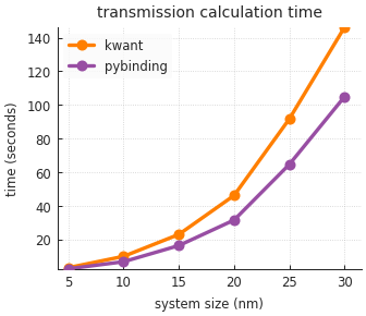
For each system size, the transmission is calculated as a function of barrier height for 100 values. Even though pybinding reconstructs the entire model every time the barrier is changed, the system build time is so fast that it doesn’t affect the total calculation time. In fact, the extremely fast build actually enables pybinding to outperform Kwant in the overall calculation. Even though Kwant only repopulates field data at each loop iteration, this still takes more time than it does for pybinding to fully reconstruct the system.
Note that this example presents a relatively simple system with a square barrier. This is done to keep the run time to only a few minutes, for convenience. Here, pybinding speeds up the overall calculation by about 40%. For more realistic examples with larger scattering regions and complicated field functions with multiple parameters, a speedup of 3-4 times can be achieved by using pybinding’s model builder.
Floating-point precision
Pybinding can generate the Hamiltonian matrix with one of four data types: real or complex numbers
with single or double precision (32-bit or 64-bit floating point). The selection is dynamic. The
starting case is always real with single precision and from there the data type is automatically
promoted as needed by the model. For example, adding translationally symmetry or a magnetic field
will cause the builder to switch to complex numbers – this is detected automatically. On the other
hand, the switch to double precision needs to be requested by the user. The onsite and hopping
energy modifiers have an optional is_double parameter which can be set to
True. The builder switches to double precision if requested by at least one modifier.
Alternatively, force_double_precision() can be given to a Model as a direct
parameter.
The reason for all of this is performance. Most solvers work faster with smaller data types: they
consume less memory and bandwidth and SIMD vectorization becomes more efficient. This is assuming
that single precision and/or real numbers are sufficient to describe the given model. In case of
Kwant’s solvers, it seems to require double precision in most cases. This is the reason for the
is_double=True flag in the above example. Keep this in mind when exporting to Kwant.