Model structure
A structure plot presents the crystal structure of a model by drawing lattice sites as circles and hoppings as lines which connect the circles. At first glance, this seems like a combination of the standard scatter and line plots found in matplotlib, but the specific requirements of tight-binding complicate the implementation. This is why pybinding has its own specialized structure plotting functions. While these functions are based on matplotlib, they offer additional options which will be explained here.
Download this page as a Jupyter notebook
Structure plot classes
A few different classes in pybinding use structure plots. These are Lattice,
Model, System, Lead and StructureMap. They all represent
some kind of spatial structure with sites and hoppings. Note that most of these classes are
components of the main Model. Calling their plot methods will draw the structure which
they represent. The following pseudo-code presents a few possibilities:
model = pb.Model(...)  # specify model
model.attach_lead(...)  # specify leads

model.lattice.plot()  # just the unit cell
model.plot()  # the main system and leads
model.system.plot()  # only the main system
model.leads[0].plot()  # only lead 0
In the following sections we’ll present a few features of the structure plotting API. The examples
will involve mainly Model.plot(), but all of these methods share the same common API.
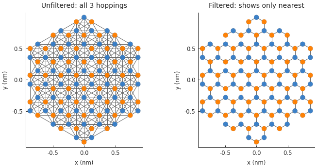
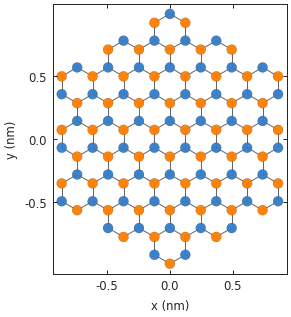
Draw only certain hoppings
The structure plot usually draws lines for all hoppings. We can see an example here with the
third-nearest-neighbor model of graphene. Note the huge number of hoppings in the figure below.
The extra information may be useful for calculations, but it is not always desirable for figures
because of the extra noise. To filter out some of the lines, we can pass the draw_only argument
as a list of hopping names. For example, if we only want the first-nearest neighbors:
from pybinding.repository import graphene

plt.figure(figsize=(7, 3))
model = pb.Model(graphene.monolayer(nearest_neighbors=3), graphene.hexagon_ac(1))

plt.subplot(121, title="Unfiltered: all 3 hoppings")
model.plot()

plt.subplot(122, title="Filtered: shows only nearest")
model.plot(hopping={'draw_only': ['t']})
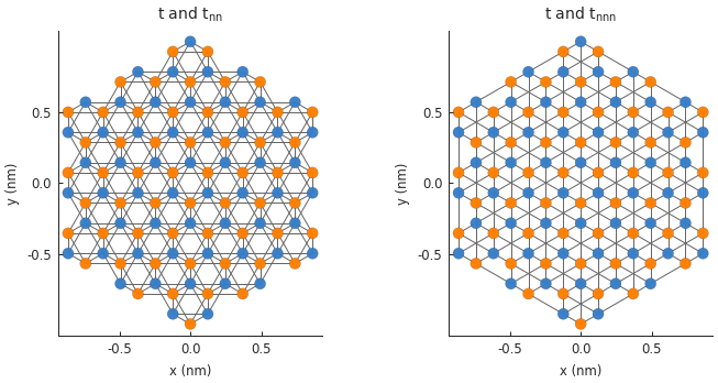
We can also select hoppings in any combination:
plt.figure(figsize=(7, 3))

plt.subplot(121, title="$t$ and $t_{nn}$")
model.plot(hopping={'draw_only': ['t', 't_nn']})

plt.subplot(122, title="$t$ and $t_{nnn}$")
model.plot(hopping={'draw_only': ['t', 't_nnn']})
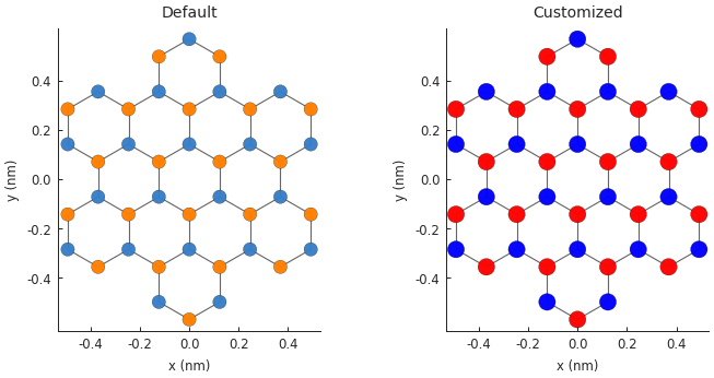
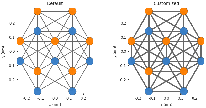
Site radius and color
The site radius is given in data units (nanometers in this example). Colors are passed as a list of colors or a matplotlib colormap.
plt.figure(figsize=(7, 3))
model = pb.Model(graphene.monolayer(), graphene.hexagon_ac(0.5))

plt.subplot(121, title="Default")
model.plot()

plt.subplot(122, title="Customized")
model.plot(site={'radius': 0.04, 'cmap': ['blue', 'red']})
Hopping width and color
By default, all hopping kinds (nearest, next-nearest, etc.) are shown using the same line color,
but they can be colorized using the cmap parameter.
plt.figure(figsize=(7, 3))
model = pb.Model(graphene.monolayer(nearest_neighbors=3), pb.rectangle(0.6))

plt.subplot(121, title="Default")
model.plot()

plt.subplot(122, title="Customized")
model.plot(hopping={'width': 2, 'cmap': 'auto'})
Redraw all axes spines
By default, pybinding plots will remove the right and top axes spines. To recover those lines
call the pltutils.respine() function.
model = pb.Model(graphene.monolayer(), graphene.hexagon_ac(1))
model.plot()
pb.pltutils.respine()
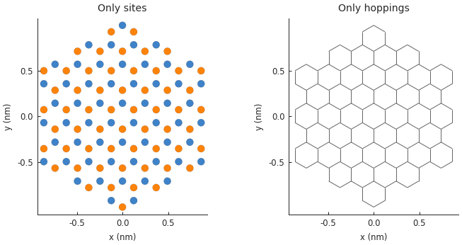
Plot only sites or only hoppings
It can sometimes be useful to separate the plotting of sites and hoppings. Notably, for large systems drawing a huge number of hopping lines can become quite slow and they may even be too small to actually see in the figure. In such cases, removing the hoppings can speed up plotting considerably. Another use case is for the composition of multiple plots – see the next page for an example.
plt.figure(figsize=(7, 3))
model = pb.Model(graphene.monolayer(), graphene.hexagon_ac(1))

plt.subplot(121, title="Only sites")
model.plot(hopping={"width": 0})

plt.subplot(122, title="Only hoppings")
model.plot(site={"radius": 0})
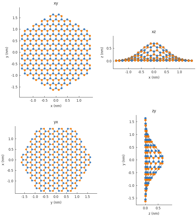
Rotating the view
By default, all structure plots show the xy-plane. The view can be rotated by settings the axes
argument to a string consisting of any combination of the letters “x”, “y” and “z”.
model = pb.Model(graphene.monolayer().with_offset([-graphene.a / 2, 0]),
                 pb.regular_polygon(num_sides=6, radius=1.8),
                 graphene.gaussian_bump(height=0.7, sigma=0.7))

plt.figure(figsize=(6.8, 7.5))
plt.subplot(221, title="xy", ylim=[-1.8, 1.8])
model.plot()
plt.subplot(222, title="xz")
model.plot(axes="xz")
plt.subplot(223, title="yx", xlim=[-1.8, 1.8])
model.plot(axes="yx")
plt.subplot(224, title="zy")
model.plot(axes="zy")
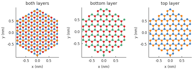
Slicing layers
For multilayer materials, it is sometimes useful to plot each layer individually.
model = pb.Model(graphene.bilayer().with_offset([graphene.a/2, 0]),
                 pb.regular_polygon(num_sides=6, radius=1))

plt.figure(figsize=(6.8, 1.8))
plt.subplot(131, title="both layers")
model.plot()

plt.subplot(132, title="bottom layer")
s = model.system
s[s.z < 0].plot()

plt.subplot(133, title="top layer")
s[s.z >= 0].plot()